Language Modeling

Technical Program Session SPE-4

CAPITALIZATION NORMALIZATION FOR LANGUAGE MODELING WITH AN ACCURATE AND EFFICIENT HIERARCHICAL RNN MODEL

Google Research

Problem

Capitalization normalization (truecasing) is the task of restoring the correct case (uppercase or lowercase) of noisy text.

Proposed method

A fast, accurate and compact two-level hierarchical word-and-character-based RNN

Used the truecaser to normalize user-generated text in a Federated Learning framework for language modeling.

Key Findings

In a real user A/B experiment, authors demonstrated that the improvement translates to reduced prediction error rates in a virtual keyboard application.

NEURAL-FST CLASS LANGUAGE MODEL FOR END-TO-END SPEECH RECOGNITION

Facebook AI, USA

Proposed method

Neural-FST Class Language Model (NFCLM) for endto-end speech recognition

a novel method that combines neural network language models (NNLMs) and finite state transducers (FSTs) in a mathematically consistent framework

Key Findings

NFCLM significantly outperforms NNLM by 15.8% relative in terms of WER.

NFCLM achieves similar performance as traditional NNLM and FST shallow fusion while being less prone to overbiasing and 12 times more compact, making it more suitable for on-device usage.

ENHANCE RNNLMS WITH HIERARCHICAL MULTI-TASK LEARNING FOR ASR

University of Missouri, USA

Proposed method

Key Findings

RESCOREBERT: DISCRIMINATIVE SPEECH RECOGNITION RESCORING WITH BERT

1Amazon Alexa AI, USA 2Emory University, USA

Problem

Second-pass rescoring improves the outputs from a first-pass decoder by implementing a lattice rescoring or n-best re-ranking.

Proposed method (RescoreBERT)

Authors showed how to train a BERT-based rescoring model with minimum WER (MWER) loss, to incorporate the improvements of a discriminative loss into fine-tuning of deep bidirectional pretrained models for ASR.

Authors proposed a fusion strategy that incorporates the MLM into the discriminative training process to effectively distill knowledge from a pretrained model. We further propose an alternative discriminative loss.

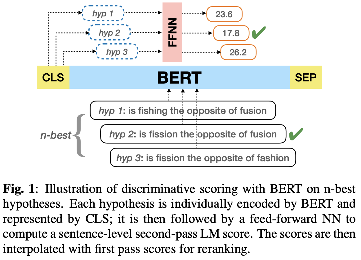
Key Findings

Reduced WER by 6.6%/3.4% relative on the LibriSpeech clean/other test sets over a BERT baseline without discriminative objective

Found that it reduces both latency and WER (by 3 to 8% relative) over an LSTM rescoring model.

Hybrid sub-word segmentation for handling long tail in morphologically rich low resource languages

Cognitive Systems Lab, University Bremen, Germany

Problem

Dealing with Out Of Vocabulary (OOV) words or unseen words

For morphologically rich languages having high type token ratio, the OOV percentage is also quite high.

Sub-word segmentation has been found to be one of the major approaches in dealing with OOVs.

Proposed method 

This paper presents a hybrid sub-word segmentation algorithm to deal with OOVs.

A sub-word segmentation evaluation methodology is also presented.

All the experiments are done for conversational code-switched Malayalam-English corpus.

Speech Recognition: Robust Speech Recognition I

Technical Program Session SPE-2

AUDIO-VISUAL MULTI-CHANNEL SPEECH SEPARATION, DEREVERBERATION AND RECOGNITION

The Chinese University of Hong Kong; Tencent AI lab

Problem

accurate recognition of cocktail party speech characterised by the interference from overlapping speakers, background noise and room reverberation.

Proposed method

In this paper, an audiovisual multi-channel speech separation, dereverberation and recognition approach with visual information into all three stages of the system is proposed.

The advantage of the additional visual modality over using audio only is demonstrated on two neural dereverberation approaches based on DNN-WPE and spectral mapping respectively.

BEST OF BOTH WORLDS: MULTI-TASK AUDIO-VISUAL AUTOMATIC SPEECH RECOGNITION AND ACTIVE SPEAKER DETECTION

Google, Inc.

Problem

Under noisy conditions, automatic speech recognition (ASR) can greatly benefit from the addition of visual signals coming from a video of the speaker’s face.

현실적으로 여러 얼굴이 존재하는 경우가 많은데 전통적으로 active speaker detection (ASD)으로  모든 시간마다 audio와 일치하는 active speaker's face를 분리하는 모델을 따로 사용했으나, 최근에는 attention 모델을 추가해서 별도의 ASD를 설계하지 않고 audio와 모든 face candidate을  모델에 집어 넣어 end-to-end way로 처리 하기도 한다.

Proposed method

2.1. A/V Backbone: Shared Audio-Visual Frontend

Acoustic Features. log mel filterbank

Audio and Video Synchronization. resample video

Visual Features. ConvNet on top of the synchronized video

Attention Mechanism. in order to soft-select the one matching the audio.

2.2. ASR Model - Transformer-Transducer Model

For ASR, the weighted visual features and input acoustic features are then concatenated along the last dimension, producing audio-visual features which are then fed to the ASR encoder.

2.3. ASD Model

For ASD, the attention scores is used directly for the model prediction. For each audio query and each timestep, the attention scores give a measure of how well each candidate video corresponds to the audio.

3. MULTI-TASK LOSS FOR A/V ASR AND ASD

ASD. For active speaker detection, the normalized attention weights can be used to train the attention module directly with cross entropy loss.

ASR. RNN-T loss

MTL Loss. We combine the ASD and ASR losses with a weighted linear sum of the losses 

Key Findings

This paper presents a multi-task learning (MTL) for a model that can simultaneously perform audio-visual ASR and active speaker detection, improving previous work on multiperson audio-visual ASR.

Combining the two tasks is enough to significantly improve the performance of the model in the ASD task relative to the baseline.

IMPROVING NOISE ROBUSTNESS OF CONTRASTIVE SPEECH REPRESENTATION LEARNING WITH SPEECH RECONSTRUCTION

The Ohio State University, USA, Microsoft Corporation

Problem

Noise Robust ASR

Proposed method

In this paper, authors employ a noise-robust representation learned by a refined self-supervised framework of wav2vec 2.0 for noisy speech recognition. They combine a reconstruction module with contrastive learning and perform multi-task continual pre-training to explicitly reconstruct the clean speech from the noisy input.

음성 데이터 관련해서 맨날 까먹고 헷갈리는 간단한 내용에 대해 메모합니다.

만약 이런 질문이 있다면, 어떤식으로 계산할 수 있을까요?

16kH, 16 Bit인 Wave 파일들 여러개의 총 용량이 500GB 일 때, 해당 Wav 파일들의 총 몇시간인가?

우선 단위에 대해서 정리를 해보겠습니다.

1) 연산 단위
1 KByte = 1024 Byte
1 MByte = 1024 KByte
1 GByte = 1024 MByte

2) 샘플링 레이트 (Sampling Rate)
1 KHz = 1024 Hz (초당 1024 Byte)
16 KHz = 16 * 1024 Hz (초당 16 * 1024 Byte)

3) 비트 레이트 (Bit Rate)
16 Bit = 2 Byte

이제 16kH, 16 Bit인 Wave 1초짜리 용량이 어떻게 되는지 계산해보면 다음과 같습니다.

2 Byte (16 bit) X 16 * 1024 Byte ( 초당 16 * 1024 Hz) = 32 Kb / 1 sec

따라서 1 sec, 1 min, 1 hour 데이터 용량은 다음과 같습니다.

32 KB | 1 sec
1.92 MB = 32 kb X 60 | 1 min
115.2 MB = 1.92 Mb X 60 | 1 hour

결론적으로 답은?!

500 X 1024 MByte / 115.2 Mb (1H) = 4444 H = 185 일

음성인식을 위해 일반적으로 16kHz, 16-bit 인 Wave 파일을 많이 다루니, 

대략적으로 음성데이터는 1초에 32 KB, 1분에 2MB, 그리고 1 시간에 115 MB 사이즈 정도 된다고 외우고 있으면 좋을 듯 합니다!

개요

음성 인식, 음성 합성, 오디오 신호 처리 등의 기술을 익히기 위해서는 신호에 대한 기본적인 지식과 컴퓨터 상에서 다룰 수 있는 능력이 있어야 합니다. 신호는 시간 영역과 주파수 영역에서 분석할 수 있으며 파이썬으로 Librosa 라이브러리를 사용하여 손쉽게 분석이 가능합니다.

오디오 파일 Load

오디오 파일은 일반적으로 wav, pcm 등의 형식으로 저장되며 sampling 개념을 사용하여 디지털화 됩니다. 오디오 데이터 처리를 위해 대표적으로 사용하는 Python 라이브러리는 librosa 입니다. librosa를 사용하여, 오디오 파일을 로드 해보겠습니다.

import librosa

audio_data = 'example.wav'

# 오디오 파일은 명시된 특정 샘플 속도 (sr)로 샘플링 된 후 NumPy 배열로 load 된다.
x = librosa.load(audio_data, sr=16000)

The sampling rate (sr) 는 sound의 초당 sample (data points) 수 입니다. 예를 들어 sampling frequency가 44kHz 인 경우 60 초 길이의 파일은 2,646,000(44000*60) 개의 샘플로 구성되어 있습니다.

시간 영역(TIme-domain) 에서 분석

일반적으로 음성/오디오 신호는 시간영역과 주파수영역에서 분석을 할 수 있습니다. 위에서 메모리 상에 load한 샘플링된 신호(데이터)를 시간영역에서 시간에 따른 파형의 진폭을 표현 해보겠습니다.

신호를 시각화하고 plotting 하기 위해 Python 시각화 대표 라이브러리인 Matplotlib 를 사용합니다.

import matplotlib.pyplot as plt
import librosa.display

plt.figure(figsize=(14, 5))

librosa.display.waveplot(x, sr=16000)

주파수 영역(Frequency-domain) 에서 분석

다음으로 주파수 영역에서 신호를 그려보겠습니다.

spectrogram을 사용하면 시간에 따라 주파수 스펙트럼이 어떻게 변화하는지 확인할 수 있습니다.

spectrogram : 시간에 따라 변화하는 신호의 주파수 스펙트럼의 크기를 시각적으로 표현한 것

librosa 라이브러리에 포함되어 있는 "Short Time Fourier Transform (STFT)" 를 사용하여 시간영역의 값을 주파수 영역에서 표현한 것입니다. STFT를 통해 구할 수 있는 값은 magnitude, phase로 나눌 수 있고, spectrogram은 magnitude만 가지고, 시간축에 대해서 표현하는 것입니다. abs()함수를 통해 magnitude를 구한후 db scale로 변경하여 다음과 같이 시간에 따른 스펙트럼의 크기를 확인할 수 있습니다.

X = librosa.stft(x)

X_mag = abs(X)

# energy levels(dB) 로 변경
Xdb = librosa.amplitude_to_db(X_mag)

plt.figure(figsize=(20, 5))
librosa.display.specshow(Xdb, sr=16000, x_axis='time', y_axis='hz')
plt.colorbar()

개요

오늘은 "SUDO RM -RF: EFFICIENT NETWORKS FOR UNIVERSAL AUDIO SOURCE SEPARATION [1]" 논문에 대해서 내 마음대로 간단하게 메모를 하려고 한다. 1저자는 Efthymios Tzinis이고, 최근 source separation 모델에 대해서 열심히 연구 중인 분이다.

최근 source separation 분야에서는 time domain에서 end-to-end 로 처리를 하는 알고리즘들이 주류를 이루고 있다. ConvTasNet, DPRNN, two-step approach 등, source separation 의 성능을 계속해서 개선해나가고 있는데,

오늘 볼 논문에서 소개하는 "SUDO RM -RF" 알고리즘은 적은 자원을 이용해서 빠르게, 좋은 separation 성능을 낼 수 있는 알고리즘에 관한 것이다.

알고리즘의 구조

먼저 전체적인 알고리즘의 구조는 간단하다. 

1. 크게 Encoder, Separator, Decoder로 구성되어 있다. STFT 대신 encoder, decoder를 구조를 사용하여 음성신호를 Latent space 에서 가지고 논다.

2. time domain 신호를 encoder를 태우고, 나온 latent representation을 separation module (SM)을 태운다. SM의 목적은 source들의 mask들을 추정하기 위함이다.

3. 추정된 mask들과 encoder에서 나온 latent representation 를 element-wise 곱을 시킨 후 나온 각각의 reconstructed latent representation들을 decoder를 태워서, 분리된 time domain 신호들을 얻는다.

전체적인 그림은 다음과 같다.

separator module

이 알고리즘의 핵심인 separator module을 조금 더 자세히 살펴보자.

1. point-wise conv로 encoded mixture representation을 project 시키고, layer-normalization (LN)을 통해 각 채널마다 temporal dimension에 대해서 norm을 한다.

2. 그 후, non-linear transformations을 수행하는데, 저자들은 이 부분을 U-convolutional block 이라고 명명해놓았다. U-convolutional block의 아키텍처와 세부 알고리즘 설명은 다음과 같다.

• multiple resolution으로 부터 정보를 추출하여 활용하는 U-Net 구조를 사용하였다.
• depth-wise conv 는 downsampling 과정에 넣었고, 그 덕분에 연산량이 상당히 줄어든 듯 하다.

3. U-convolutional block 통해 나온 representationd을 소스의 개수만큼 1D conv를 태우는데, 이 단계는 저자들의 이전 연구에서 소개되었고, y^B후 바로 activation을 사용하는 것보다 학습 측면에서 안정적이기에 도입했다고 한다.

4. z^(1), z^(2)를 기반으로 softmax를 적용하여 masks를 추정한다.

REFERENCE

[1] https://arxiv.org/pdf/2007.06833.pdf

microphones과 loudspeakers 사이의 acoutic coupling에 의해서 발생되는 Acoustic echo는 음성 통신의 품질을 굉장히 좋지 않게 만든다. 이러한 acoustic echo 문제를 해결하기 위한 분야가 Acoustic echo cancellation (AEC), acoustic echo suppression (AEC) 인데, 일반적으로 Time/Frequency 도메인에서 linear adaptive filter (NLMS, and etc) 사용하고, 다른 여러 방법이 존재한다.

하지만 far-end power amplifier/far-end loudspeakers/non-linear echo path(transfer function)/ imperfect AEC 등에 의해 nonlinearity 가 반영되기 때문에, 단순한 linear filtering 접근 방법으로는 acoustic echo를 완전히 제거할 수 없다는 한계가 존재한다. 이러한 nonlinear echo 성분들을 제거하기 위해서 residual echo suppression (RES) 모듈을 이용해서 잔여 echo를 추가로 제거한다. 

일반적인 에코제거 관련 문제를 좀 더 정확하게 이해하기 위해 그림, 수식을 첨부한다.

Acoustic echo, caused by the acoustic coupling between microphones and loudspeakers, significantly degrades the quality of voice communication. The fields of Acoustic Echo Cancellation (AEC) and Acoustic Echo Suppression (AES) address this problem, typically employing linear adaptive filters (like NLMS) in the Time/Frequency domain, among other methods.

However, there are limitations due to nonlinearity introduced by factors such as far-end power amplifiers, far-end loudspeakers, nonlinear echo paths (transfer functions), and imperfect AEC, which means simple linear filtering approaches can't completely eliminate acoustic echo. To mitigate these nonlinear echo components, a Residual Echo Suppression (RES) module is used to further reduce the remaining echo.

For a more precise understanding of the issues related to echo removal, diagrams and equations are often included.

y(t) = s(n) + d(n) + v(n)

d^(n) = h^(n) * x(n)

s_AEC(n) = y(n) - d^(n)

s_AEC(n) = e(n) = y(n) - d^(n) =  [ d(n) + s(n) + v(n) ] - d^(n)

y(n) : microphone signal

d(n) : echo signal

s(n) : near-end speech

v(n) : background noise

e(n) : AEC output signal

d^(n) : linear echo estimate produced by an AEC filter

x(n) : Far-end signal

h^(n) : adaptive filter

* : convolution operation

Speech Sentiment Analysis via Pre-Trained Features from End-to-End ASR Models, ICASSP 2020, USC(intern), Google

Fusion Approaches for Emotion Recognition from Speech Using Acoustic and Text-Based Features, 

1) Text-based Model

- BERT에서 추출한 768 dim Lexical feature를 text-based 기본 feature로 사용

- 1 conv1d : embedding layer for reducing dimension (from 768 to 128)

- 2 conv1d : for relationships across neighboring elemnets of the sequence.

- Mean Pooling over time

- softmax layer

2) Audio-based Model

- 36 dim acoustic feature(pitch, jitter, shimmer, logHNR, loudness, 13-MFCC, and first orders) 를 기본 feature로 사용 

- 2 conv1d : for the temporal evolution of the input sequence

- mean-pooling over time

- softmax layer

3) Fusion Models

- Text-based Model, Audio-based Model 을 동시에 jointly하게 학습 시키는 방법

- Text-based Model, Audio-based Model 을 각각 학습을 시키고, 학습된 W를 밑에 단계부터 fix시켜 놓고 학습을 추가로 하는 방법 등

개요

이번 글에서는 16 비트 고정 소수점(16-bit fixed point), 24 비트 고정 소수점(24-bit fixed poin), 32 비트 부동 소수점(32-bit floating point) 오디오 파일의 차이에 대해 설명한다.

16-bit fixed point WAV File

기존의 16비트 WAV 파일은 압축되지 않은 오디오 샘플을 저장하며, 각 샘플들은 16 자리(이진수 = "Bit")의 이진수로 표현된다.

이 숫자들은 정수(소수점이 없는)이기 때문에 "Fixed-Point"이다. 이진 형식의 16비트 번호는 0에서 65535(2^16)까지의 정수를 나타낸다.

이 숫자 값은 signal amplitude에 해당하는 discrete voltage level을 나타낸다.

65535는 신호가 될 수 있는 최대 amplitude(loudest)을 나타내며, 가장 낮은 값은 파일의 noise floor를 나타내며, 가장 낮은 비트는 0과 1 사이에서 왔다갔다 한다. 65536 레벨이 있으므로, noise는 = (1/65536) 이다.

이 노이즈를 dB 형식으로 설정하면 the noise level 과 maximum levels은 각각 다음과 같다.

dBnoise = 20 x log (1/65536) = -96.3 dB 
dBmax = 20 x log (65536/65536) = 0 dB

16-bit WAV 파일로 표현할 수 있는, 최대 dynamic 범위는 다음과 같다.

(0 dB – (-96.3 dB)) = 96.3 dB 

따라서 16 비트 WAV 파일은 0dBFS에서 -96dBFS까지 오디오를 저장할 수 있다.

각 오디오 샘플은 하드디스크 또는 메모리에서 16 bit의 공간을 차지하며 48kHz sampling rate에서 mono-channel 16 bit, 48kHz 파일을 저장하려면 초당 16 x 48,000 = 768,000 비트가 필요하다.

24-bit fixed point WAV File

24-bit (fixed point) WAV 파일은 16 bit word를 확장하여 50 % 더 많은 bit를 추가하여 amplitude resolution를 향상시킨다.

높은 bit 일수록, 오디오 신호를 나누기 위한 더 많은 discrete voltage levels 이 있다. 이진 표기법의 24-bit 범위는 0 - 16,777,215 (2^24)이다.

또한, the noise level 과 maximum levels은 각각 다음과 같다.

dBnoise = 20 x log (1/16777216) = -144.5 dB

dBmax = 20 x log (16777216/16777216) = 0 dB

 24-bit (fixed point) 의 dynamic 범위는 다음과 같다.

(0 dB – (-144.5 dB)) = 144.5 dB

따라서 16 비트 WAV 파일은 0dBFS에서 -144.5dBFS까지 오디오를 저장할 수 있다.

16-bit 파일과 마찬가지로, 24-bit wav 파일이 감당할 수 있는 가장 큰 신호는, 0 dBFS이다. 

각 오디오 샘플은 하드디스크 또는 메모리에서 24 bit의 공간을 차지하며 48kHz sampling rate에서 mono-channel 24 bit, 48kHz 파일을 저장하려면 초당 24 x 48,000 = 1,152,000 비트가 필요하다.

16 비트 파일에 비해 저장 공간이 50 % 증가하고 동적 범위는 96dB에서 최대 144dB로 증가하여 성능이 향상된다. 현재 24 비트, 48kHz WAV 파일은 전문 오디오 커뮤니티에서 가장 널리 사용되는 파일이다.

32-bit floating point WAV File

fixed-point 파일 (16 비트 또는 24 비트)과 비교하여 32-bit float 파일은 부동 소수점 형식으로 숫자를 저장한다.

이러한 WAV 파일의 숫자는 소수점과 지수 (예 : "1456300"대신 "1.4563 x 106")를 사용하여 "scientific notation"으로 저장되므로, 고정 소수점과 근본적으로 다르다. floating point는 fixed-point 표현에 비해 훨씬 크고 작은 숫자를 표현할 수 있다.

32-bit float 단어의 형식과 인코딩은 직관적이지 않으므로 컴퓨터가 사람이 읽을 수있는 것이 아니라, 일반적인 수학 기능을 수행 할 수 있도록 최적화되었다.

[첫 번째 Bit]는 양수 또는 음수 값을 나타내고, [다음 8 Bit]는 지수(exponent)를 나타내고 [마지막 23 Bit]는 가수(mantissa)를 나타낸다.

The largest number which can be represented is ~3.4 x 1038, and the smallest number is ~1.2 x 10-38.

가장 큰 수는 ~3.4 x 10^38

가장 작은 수는 ~1.2 x 10^-38 로 표현 가능하다.

그러므로 32-bit float WAV로 표현할 수 있는 dB는 다음과 같다.

dBnoise = 20 x log (1.2 x 10-38) = -758 dB

dBmax = 20 x log (3.4 x 1038) = 770 dB

32-bit floating point 파일로 나타낼 수 있는 dynamic range는 1528dB 이다. 지구의 sound pressure의 가장 큰 차이는 무반향실(anechoic chamber)에서 거대한 충격파(massive shockwave)에 이르기까지 약 210dB 일 수 있으므로, 1528dB는 컴퓨터 파일에서 음향 사운드 진폭을 나타내는 데 필요한 것보다 훨씬 더 크다.

32-bit floating point wav file은 ultra-high-dynamic-range를 갖는다. 24 비트 또는 16 비트 파일과 비교할 때, 32-bit floating 파일은 최대 +770dBFS이고, noise level도 굉장히 큰 range를 갖는다.

32-bit float 파일의 각 오디오 샘플은 하드 디스크 또는 메모리에서 32 bit의 공간을 소비하며 48kHz sampling rate의 경우 32 비트, 48kHz 파일에 초당 32 x 48,000 = 1,536,000 bit가 필요하다. 따라서 24 bit 파일에 비해 33 % 더 많은 저장 공간을 확보하기 위해 캡처 된 dynamic range는 144dB에서 기본적으로 무한 (1500dB 이상)까지 증가한다. 

REFERENCE

[1] https://www.sounddevices.com/32-bit-float-files-explained