오늘은 "SUDO RM -RF: EFFICIENT NETWORKS FOR UNIVERSAL AUDIO SOURCE SEPARATION [1]" 논문에 대해서 내 마음대로 간단하게 메모를 하려고 한다. 1저자는 Efthymios Tzinis이고, 최근 source separation 모델에 대해서 열심히 연구 중인 분이다.
최근 source separation 분야에서는 time domain에서 end-to-end 로 처리를 하는 알고리즘들이 주류를 이루고 있다. ConvTasNet, DPRNN, two-step approach 등, source separation 의 성능을 계속해서 개선해나가고 있는데,
오늘 볼 논문에서 소개하는 "SUDO RM -RF" 알고리즘은 적은 자원을 이용해서 빠르게, 좋은 separation 성능을 낼 수 있는 알고리즘에 관한 것이다.
알고리즘의 구조
먼저 전체적인 알고리즘의 구조는 간단하다.
1. 크게 Encoder, Separator, Decoder로 구성되어 있다. STFT 대신 encoder, decoder를 구조를 사용하여 음성신호를 Latent space 에서 가지고 논다.
2. time domain 신호를 encoder를 태우고, 나온 latent representation을 separation module (SM)을 태운다. SM의 목적은 source들의 mask들을 추정하기 위함이다.
3. 추정된 mask들과 encoder에서 나온 latent representation 를 element-wise 곱을 시킨 후 나온 각각의 reconstructed latent representation들을 decoder를 태워서, 분리된 time domain 신호들을 얻는다.
전체적인 그림은 다음과 같다.
separator module
이 알고리즘의 핵심인 separator module을 조금 더 자세히 살펴보자.
1. point-wise conv로 encoded mixture representation을 project 시키고, layer-normalization (LN)을 통해 각 채널마다 temporal dimension에 대해서 norm을 한다.
2. 그 후, non-linear transformations을 수행하는데, 저자들은 이 부분을 U-convolutional block 이라고 명명해놓았다. U-convolutional block의 아키텍처와 세부 알고리즘 설명은 다음과 같다.
multiple resolution으로 부터 정보를 추출하여 활용하는 U-Net 구조를 사용하였다.
depth-wise conv 는 downsampling 과정에 넣었고, 그 덕분에 연산량이 상당히 줄어든 듯 하다.
3. U-convolutional block 통해 나온 representationd을 소스의 개수만큼 1D conv를 태우는데, 이 단계는 저자들의 이전 연구에서 소개되었고, y^B후 바로 activation을 사용하는 것보다 학습 측면에서 안정적이기에 도입했다고 한다.
microphones과 loudspeakers 사이의 acoutic coupling에 의해서 발생되는 Acoustic echo는 음성 통신의 품질을 굉장히 좋지 않게 만든다. 이러한 acoustic echo 문제를 해결하기 위한 분야가 Acoustic echo cancellation (AEC), acoustic echo suppression (AEC) 인데, 일반적으로 Time/Frequency 도메인에서 linear adaptive filter (NLMS, and etc) 사용하고, 다른 여러 방법이 존재한다.
하지만 far-end power amplifier/far-end loudspeakers/non-linear echo path(transfer function)/ imperfect AEC 등에 의해 nonlinearity 가 반영되기 때문에, 단순한 linear filtering 접근 방법으로는 acoustic echo를 완전히 제거할 수 없다는 한계가 존재한다. 이러한 nonlinear echo 성분들을 제거하기 위해서 residual echo suppression (RES) 모듈을 이용해서 잔여 echo를 추가로 제거한다.
일반적인 에코제거 관련 문제를 좀 더 정확하게 이해하기 위해 그림, 수식을 첨부한다.
Acoustic echo, caused by the acoustic coupling between microphones and loudspeakers, significantly degrades the quality of voice communication. The fields of Acoustic Echo Cancellation (AEC) and Acoustic Echo Suppression (AES) address this problem, typically employing linear adaptive filters (like NLMS) in the Time/Frequency domain, among other methods.
However, there are limitations due to nonlinearity introduced by factors such as far-end power amplifiers, far-end loudspeakers, nonlinear echo paths (transfer functions), and imperfect AEC, which means simple linear filtering approaches can't completely eliminate acoustic echo. To mitigate these nonlinear echo components, a Residual Echo Suppression (RES) module is used to further reduce the remaining echo.
For a more precise understanding of the issues related to echo removal, diagrams and equations are often included.
이번 글에서는 16 비트 고정 소수점(16-bit fixed point), 24 비트 고정 소수점(24-bit fixed poin), 32 비트 부동 소수점(32-bit floating point) 오디오 파일의 차이에 대해 설명한다.
16-bit fixed point WAV File
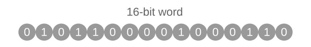
기존의 16비트 WAV 파일은 압축되지 않은 오디오 샘플을 저장하며, 각 샘플들은 16 자리(이진수 = "Bit")의 이진수로 표현된다.
이 숫자들은 정수(소수점이 없는)이기 때문에 "Fixed-Point"이다. 이진 형식의 16비트 번호는 0에서 65535(2^16)까지의 정수를 나타낸다.
이 숫자 값은 signal amplitude에 해당하는 discrete voltage level을 나타낸다.
65535는 신호가 될 수 있는 최대 amplitude(loudest)을 나타내며, 가장 낮은 값은 파일의 noise floor를 나타내며, 가장 낮은 비트는 0과 1 사이에서 왔다갔다 한다. 65536 레벨이 있으므로, noise는 = (1/65536) 이다.
이 노이즈를 dB 형식으로 설정하면 the noise level 과 maximum levels은 각각 다음과 같다.
dBnoise = 20 x log (1/65536) = -96.3 dB dBmax = 20 x log (65536/65536) = 0 dB
16-bit WAV 파일로 표현할 수 있는, 최대 dynamic 범위는 다음과 같다.
(0 dB – (-96.3 dB)) = 96.3 dB
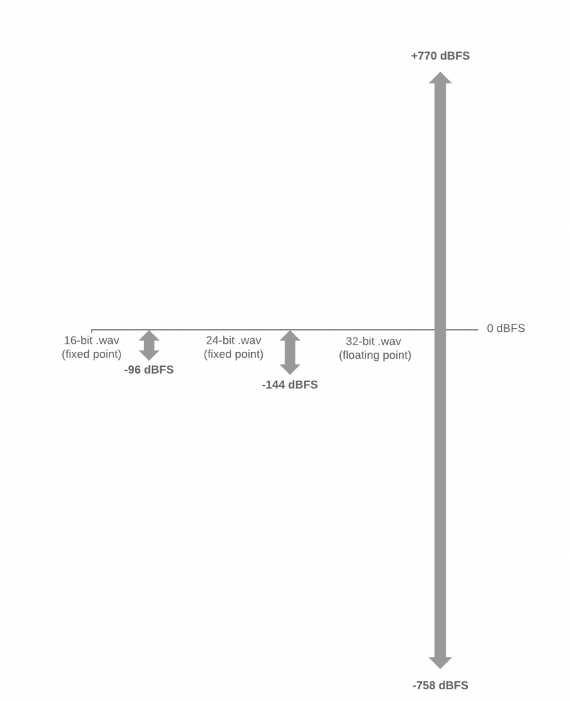
따라서 16 비트 WAV 파일은 0dBFS에서 -96dBFS까지 오디오를 저장할 수 있다.
각 오디오 샘플은 하드디스크 또는 메모리에서 16 bit의 공간을 차지하며 48kHz sampling rate에서 mono-channel 16 bit, 48kHz 파일을 저장하려면 초당 16 x 48,000 = 768,000 비트가 필요하다.
24-bit fixed point WAV File
24-bit (fixed point) WAV 파일은 16 bit word를 확장하여 50 % 더 많은 bit를 추가하여 amplituderesolution를 향상시킨다.
높은 bit 일수록, 오디오 신호를 나누기 위한 더 많은 discrete voltage levels 이 있다. 이진 표기법의 24-bit 범위는 0 - 16,777,215 (2^24)이다.
또한, the noise level 과 maximum levels은 각각 다음과 같다.
dBnoise = 20 x log (1/16777216) = -144.5 dB
dBmax = 20 x log (16777216/16777216) = 0 dB
24-bit (fixed point) 의 dynamic 범위는 다음과 같다.
(0 dB – (-144.5 dB)) = 144.5 dB
따라서 16 비트 WAV 파일은 0dBFS에서 -144.5dBFS까지 오디오를 저장할 수 있다.
16-bit 파일과 마찬가지로, 24-bit wav 파일이 감당할 수 있는 가장 큰 신호는, 0 dBFS이다.
각 오디오 샘플은 하드디스크 또는 메모리에서 24 bit의 공간을 차지하며 48kHz sampling rate에서 mono-channel 24 bit, 48kHz 파일을 저장하려면 초당 24 x 48,000 = 1,152,000 비트가 필요하다.
16 비트 파일에 비해 저장 공간이 50 % 증가하고 동적 범위는 96dB에서 최대 144dB로 증가하여 성능이 향상된다. 현재 24 비트, 48kHz WAV 파일은 전문 오디오 커뮤니티에서 가장 널리 사용되는 파일이다.
32-bit floating point WAV File
fixed-point 파일 (16 비트 또는 24 비트)과 비교하여 32-bit float 파일은 부동 소수점 형식으로 숫자를 저장한다.
이러한 WAV 파일의 숫자는 소수점과 지수 (예 : "1456300"대신 "1.4563 x 106")를 사용하여 "scientific notation"으로 저장되므로, 고정 소수점과 근본적으로 다르다. floating point는 fixed-point 표현에 비해 훨씬 크고 작은 숫자를 표현할 수 있다.
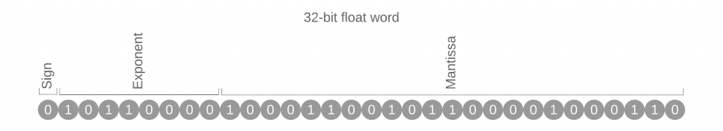
32-bit float 단어의 형식과 인코딩은 직관적이지 않으므로 컴퓨터가 사람이 읽을 수있는 것이 아니라, 일반적인 수학 기능을 수행 할 수 있도록 최적화되었다.
[첫 번째 Bit]는 양수 또는 음수 값을 나타내고, [다음 8 Bit]는 지수(exponent)를 나타내고 [마지막 23 Bit]는 가수(mantissa)를 나타낸다.
The largest number which can be represented is ~3.4 x 1038, and the smallest number is ~1.2 x 10-38.
가장 큰 수는 ~3.4 x 10^38
가장 작은 수는 ~1.2 x 10^-38 로 표현 가능하다.
그러므로 32-bit float WAV로 표현할 수 있는 dB는 다음과 같다.
dBnoise = 20 x log (1.2 x 10-38) = -758 dB
dBmax = 20 x log (3.4 x 1038) = 770 dB
32-bit floating point 파일로 나타낼 수 있는 dynamic range는 1528dB 이다. 지구의 sound pressure의 가장 큰 차이는 무반향실(anechoic chamber)에서 거대한 충격파(massive shockwave)에 이르기까지 약 210dB 일 수 있으므로, 1528dB는 컴퓨터 파일에서 음향 사운드 진폭을 나타내는 데 필요한 것보다 훨씬 더 크다.
32-bit floating point wav file은 ultra-high-dynamic-range를 갖는다. 24 비트 또는 16 비트 파일과 비교할 때, 32-bit floating 파일은 최대 +770dBFS이고, noise level도 굉장히 큰 range를 갖는다.
32-bit float 파일의 각 오디오 샘플은 하드 디스크 또는 메모리에서 32 bit의 공간을 소비하며 48kHz sampling rate의 경우 32 비트, 48kHz 파일에 초당 32 x 48,000 = 1,536,000 bit가 필요하다. 따라서 24 bit 파일에 비해 33 % 더 많은 저장 공간을 확보하기 위해 캡처 된 dynamic range는 144dB에서 기본적으로 무한 (1500dB 이상)까지 증가한다.
일반적으로 Audio source separation을 위한 모델은 spectrogram 기반 프로세싱을 많이 하고, phase 정보를 무시하고, magnitude 정보만을 가지고 처리한다.
이로 인한 한계가 있고, 최근 이를 해결하기 위한 방법으로 spectrogram-based processing이 아닌, Time-domain waveform 기반으로 하는 모델들이 나오고 있다.
그 중 대표적인 모델인 WAVE-U-NET 에 대해서 내 마음대로 간단하게 리뷰 해보고자 한다.
Wave-U-Net 아키텍처
우리의 목표는 주어진 Mixture waveform 을 2개의 Source waveform으로 나누는 것이다.
Fig 1은 Wave-U-Net 아키텍처의 다이어그램이다. 먼저 크게 2가지 부분으로 구성되어 있다. 이 두 부분은 Fig 상에서 왼쪽(노란색), 오른쪽(초록색) 부분인데, 나는 각각 이 큰 덩어리를 encoder/decoder라고 명명하고 설명하겠다.
[Fig 1] Wave-U-Net 아키텍처 다이어그램
먼저 인코더 부분은 여러 downsampling block의 연속으로 구성되어 있다. 각각의 downsampling block들은 또 2가지 모듈로 구성되어 있는데, 그것은 1D Conv 모듈/ Downsampling 모듈이다. 여기서는 1D-Conv를 통해서, Time domain에서 많은 High-level features map을 추출해 내고, downsampling을 하며 시간 단계에 대해 특정한 패턴을 따르며 time sample들을 무시하여 Time resolution을 절반으로 줄인다.
다음으로, 디코더 부분을 살펴보면, upsampling block의 연속으로 구성되어 있다. upsampling block은 이전과 비슷하게 1D Transposed Conv와 Upsampling 모듈로 구성이 되어 있다. 이 때, Conv와 여러가지 Linear interpolation등의 여러가지 보간 방법을 사용한다.
그리고 추가로, 중요한 부분은, Upsampling 경로의 각 Layer는 skip-connection을 통해 downsampling 경로의 해당 Layer에 연결된다.
다시 한번 설명하면,
Downsampling 블록을 사용하여 Time domain에서 많은 High-level features을 추출해 낸다. 이러한 기능은 Upsampling (US) 블록을 사용하여 이전에 계산 된 Local의 High-resolution features과 결합되어 예측에 사용되는 Multi-Scale 기능을 제공한다. Network에는 L개의 레벨이 있으며 각 연속 레벨은 이전 레벨의 절반 시간 분해능으로 작동한다.
이를 위해 제일 먼저 1D-Convolution를 Time domain waveform에 대해 적용한다. 논문에서는 downsampling/upsampling을 위해 각각 24 hidden conv layers with 15 filter size /12hidden conv layer with 5filter size 를 사용했다. 또한 Optimization을 위해서 batchnorm 을 적용하고, activation fucntion으로는 LeakyRelu, 마지막 layer에는 tanh를 사용한다.
Decimation 단계에서는 시간 단계에 대해 특정한 패턴을 따르며 feature(time sample)들을 무시하여 Time resolution을 절반으로 줄인다.
Upsampling 단계에서는 시간 방향으로 2 배씩 업 샘플링을 수행하기 위해 Linear Interpolation을 사용한다. 이 때, aliasing 이 생기는데, 이것을 해결하기 위한 다른 방법들을 논문의 뒤에서 추가 설명/제안 한다.
Concat (x)는 현재의 High-level feature들과 더 많은 local feature들을 연결(skip-connection)한다.
Avoiding aliasing artifacts due to upsampling
개인적으로 wave-u-net에서 알고리즘에서 가장 중요한 부분은 upsampling 시, 발생하는 alising 문제를 어떻게 해결하는 방법에 관한 것이다.
feature map을 upsampling하기 위해 일반적으로 transposed convolutions with strides 을 사용한다. 이는 aliasing 같은 artifact를 발생시킨다.
k의 필터 크기와 1이상의 stride인 Transposed convolutions은 각 원래 값 사이에 x-1만큼 0으로 채워진 feature maps에 적용된 convolutions으로 볼 수 있다. 이는 subsequent low-pass filtering 없이 0으로 interleaving하면, 최종 출력에서도 high-frequency noise가 발생한다.
해결방법 I : Linear Interpolation
그래서 upsampling을 위해 transposed strided convolutions 대신, linear interpolation을 수행하여 feature space에서 시간적 연속성을 보장 한 다음 normal 컨벌루션을 수행했다고 한다.
해결방법 II : Learned upsampling
추가 성능 개선을 위해서 wave-u-net 원 논문에서는 다른 방법도 제시한다.
upsampling을 위해 Linear interpolation은 아주 간단한 해결 방법이기에 성능이 제한될 수 있다.
왜냐하면 네트워크의 feature maps들에 사용 되는 feature spaces은 feature spaces의 두 지점 사이의 linear interpolation이 그 자체로 유용한 지점이되도록 학습되지 않았기 때문이다. 만약에 upsampling 되는 feature가 학습 가능하다면 upsampling으로 인한 성능을 더욱 향상시킬 수 있을 것이다.
이를 위해 논문에서는 학습 된 upsampling Layer을 제안한다. n 개의 time steps를 갖는 주어진 F × n feature map에 대해, 우리는 매개 변수 W 및 Sigmoid 함수 σ를 사용하여 이웃 한 feature pair f_t, f_t + 1 에 대해 interpolated feature f_t + 0.5 를 계산한다. 수식은 다음과 같다:
이것은 패딩되지 않은 크기가 2 인 F filters를 사용하는 1D convolution으로 구현 될 수 있다.
학습 된 interpolationlayer는 0.5 이외의 가중치를 가진 features의 convex한 조합을 허용하므로, 간단한 linear interpolation의 일반화로 볼 수 있다.
Prediction with proper input context and resampling
[Fig 2] a) 일반적인 wav-unet 모델, b) 제안하는 sampling 적용 모델
a) 경계에 아티팩트를 생성하기 전에 균등하게 입력 된 수의 입력이 포함 된 공통 모델이다 (Common model with an even number of inputs which are zero-padded before convolving, creating artifacts at the borders.). Decimation 후, stride 2를 사용하여 transposed convolution은 여기에서 upsampling by zero-padding intermediate and border values, 다음에 일반 Conv가 발생하여, 출력에서 high-frequency artifacts를 발생시킬 수 있다.
b) 섹션 3.2.2의 upsampling을 위한 적절한 input context와 linear interpolation을 가진 모델은 zero-padding을 사용하지 않는다. features의 수는 불균일하게 유지되므로 upsampling에는 extrapolating 값 (red arrow)이 불필요하다. 출력은 더 작지만 artifacts는 예방할 수 있다.
이전 작업에서, 입력 및 feature maps은 convolving하기 전에 0으로 채워지므로, [Fig 2a]와 같이 결과 feature map의 dimension가 변경되지 않는다.
그래서 입력 및 출력 dimensions이 동일하므로 네트워크 구현이 간단해진다. 이러한 방식으로 Zero-padding 오디오 또는 spectrogram 입력은 시작과 끝에서 무음을 사용하여 입력을 효과적으로 확장한다.
그러나, 전체 오디오 신호의 임의의 위치로부터 취해지면, boundary에서의 정보는 인공적으로된다. 즉, 이 excerpt에 대한 시간적 맥락은 전체 오디오 신호에 주어 지지만 무시되고 silent 로 가정된다.
적절한 context 정보가 없으면 네트워크는 sequence의 시작과 끝 근처에서 출력 값을 예측하기가 어렵다.
결과적으로, 전체 오디오 신호에 대한 예측을 얻기 위해 테스트 시간에 출력을 겹치지 않는 segment로 연결하면 정확한 context 정보없이 인접 출력이 생성 될 때 인접 출력이 일치하지 않을 수 있으므로 세그먼트 경계에서 audible artifacts를 생성 할 수 있다.
이것의 해결책으로, 논문에서는 padding 없이 convolutions을 사용하고, 대신 출력 예측의 크기보다 큰 mixture input을 제공하여 convolutions이 적절한 audio context에서 계산되어 출력 되도록 한다 [Fig 2b 참조].
이렇게하면 feature map size가 줄어들기 때문에, 네트워크의 가능한 출력 크기를 제한하여 feature maps이 다음 convolution에 대해 항상 충분히 클 수 있다.
또한, feature maps을 resampling 할 때, [Fig 2a] 와 같이, transposed strided convolution에 대한 featuredimensions는 정확히 절반으로 또는 두 배가된다.
그러나 이것은 반드시 경계에서 적어도 하나의 값을 삽입하는 것이고, 이 역시도 아티팩트를 생성한다.
대신, 우리는 알려진 이웃 값들 사이에서만 interpolate하고 첫 번째와 마지막 항목을 유지하여 [Fig 2b]에 표시된 것처럼 n에서 2n-1 항목을 생성하거나 그 반대로 생성합니다.
decimation 후 중간 값을 복구하기 위해, 경계 값을 동일하게 유지하면서,feature map의 dimensionality가 홀수인지 확인한다.
import sys, os, argparse
import tensorflow as tf
# for LSTMBlockFusedCell(), https://github.com/tensorflow/tensorflow/issues/23369# tf.contrib.rnn# for QRNN# ?try: import qrnn# except: sys.stderr.write('import qrnn, failed\n')'''
source is from https://gist.github.com/morgangiraud/249505f540a5e53a48b0c1a869d370bf#file-medium-tffreeze-1-py
'''# The original freeze_graph function# from tensorflow.python.tools.freeze_graph import freeze_graph # dir = os.path.dirname(os.path.realpath(__file__))defmodify_op(graph_def):"""
reference : https://github.com/onnx/tensorflow-onnx/issues/77#issuecomment-445066091
"""for node in graph_def.node:
if node.op == 'Assign':
node.op = 'Identity'if'use_locking'in node.attr: del node.attr['use_locking']
if'validate_shape'in node.attr: del node.attr['validate_shape']
if len(node.input) == 2:
# input0: ref: Should be from a Variable node. May be uninitialized.# input1: value: The value to be assigned to the variable.
node.input[0] = node.input[1]
del node.input[1]
return graph_def
deffreeze_graph(model_dir, output_node_names, frozen_model_name, optimize_graph_def=0):"""Extract the sub graph defined by the output nodes and convert
all its variables into constant
Args:
model_dir: the root folder containing the checkpoint state file
output_node_names: a string, containing all the output node's names,
comma separated
frozen_model_name: a string, the name of the frozen model
optimize_graph_def: int, 1 for optimizing graph_def via tensorRT
"""ifnot tf.gfile.Exists(model_dir):
raise AssertionError(
"Export directory doesn't exists. Please specify an export ""directory: %s" % model_dir)
ifnot output_node_names:
print("You need to supply the name of a node to --output_node_names.")
return-1# We retrieve our checkpoint fullpath
checkpoint = tf.train.get_checkpoint_state(model_dir)
input_checkpoint = checkpoint.model_checkpoint_path
# We precise the file fullname of our freezed graph
absolute_model_dir = "/".join(input_checkpoint.split('/')[:-1])
output_graph_path = absolute_model_dir + "/" + frozen_model_name
# We clear devices to allow TensorFlow to control on which device it will load operations
clear_devices = True# We start a session using a temporary fresh Graphwith tf.Session(graph=tf.Graph()) as sess:
# We import the meta graph in the current default Graph
saver = tf.train.import_meta_graph(input_checkpoint + '.meta', clear_devices=clear_devices)
# We restore the weights
saver.restore(sess, input_checkpoint)
# We use a built-in TF helper to export variables to constants
output_graph_def = tf.compat.v1.graph_util.convert_variables_to_constants(
sess, # The session is used to retrieve the weights
tf.get_default_graph().as_graph_def(), # The graph_def is used to retrieve the nodes
output_node_names.split(',') # The output node names are used to select the usefull nodes
)
# Modify for 'float_ref'
output_graph_def = modify_op(output_graph_def)
# Optimize graph_def via tensorRTif optimize_graph_def:
from tensorflow.contrib import tensorrt as trt
# get optimized graph_def
trt_graph_def = trt.create_inference_graph(
input_graph_def=output_graph_def,
outputs=output_node_names.split(','),
max_batch_size=128,
max_workspace_size_bytes=1 << 30,
precision_mode='FP16', # TRT Engine precision "FP32","FP16" or "INT8"
minimum_segment_size=3# minimum number of nodes in an engine
)
output_graph_def = trt_graph_def
# Finally we serialize and dump the output graph to the filesystemwith tf.gfile.GFile(output_graph_path, "wb") as f:
f.write(output_graph_def.SerializeToString())
print("%d ops in the final graph." % len(output_graph_def.node))
print("Saved const_graph in %s"%model_dir)
return output_graph_def
freeze_graph("model/", "output_name", "dnn.pb")
모델을 freeze 할 때, 제일 신경써야할 부분은 "output_node_names" 옵션이다. 모델을 freeze시킨 후, output으로 받고 싶은 출력 노드 이름을 이곳에 명시해줘야 한다. 이 부분을 확인할 수 있는 부분은 ".pbtxt" 파일이다. 이곳에 모든 노드 정보가 기록되므로, 이 파일을 열어서 내가 원하는 노드 네임을 찾아서 넣으면 된다.
개인적으로 노드 이름을 간단하게 확인하기 위해서, 다음 코드를 자주 활용한다.
print([print(n.name) for n in tf.get_default_graph().as_graph_def().node])
마지막으로, 또 하나의 팁을 남기자면, 모델 설계 시, 모델의 input node는 꼭 "input"로 이름을 지정해주고, 마지막 노드 또한 해당하는 텐서에 이름을 "output"으로 꼭 설정해주거나, 그렇지 못할 경우에 모델 output 부분에
tf.identity(x, name="output")
다음 코드를 추가해주면, output_node를 "output"으로 일관되게 유지할 수 있다.
Tensorflow model을 표현하기 위해서 크게 2가지 컴포넌트(Meta Graph, Checkpoint)가 필요하다.
Meta graph
.meta
tensorflow graph structure 에 대한 정보
Variables, Collection and Operations
Checkpoint
A protocol buffer with a list of recent checkpoints
weight, biases, gradients, all the variables 값
.data files: training variables 값에 대한 정보; model.ckpt.data-00000-of-00001
.index files:**checkpoint 에 대한 정보(index)
TF 1.x 버전 tf.Session()을 통해서 모델을 저장하는 코드는 다음과 같다.
with tf.Session() as sess:
    # Initializes all the variables.
    sess.run(init_all_op)
    # Runs to logit.
    sess.run(logits)
    # Creates a saver.
    saver = tf.train.Saver()
    # Save both checkpoints and meta-graph
    saver.save(sess, 'my-save-dir/my-model-10000')
    # Generates MetaGraphDef.
    saver.export_meta_graph('my-save-dir/my-model-10000.meta') #change this line
2. 전체 모델을 HDF5 파일 하나에 저장하는 방식
가중치, 모델 구성, 옵티마이저에 지정한 설정까지 파일 하나에 모두 포함된다.
model = create_model()

model.fit(train_images, train_labels, epochs=5)

# 전체 모델을 HDF5 파일로 저장합니다
model.save('my_model.h5')

# 가중치와 옵티마이저를 포함하여 정확히 동일한 모델을 다시 생성합니다
new_model = keras.models.load_model('my_model.h5')
new_model.summary()
고수준 API인 tf.keras 를 통해서 모델을 저장하고 로드하는 것은 이곳에 잘 정리되어 있다.
K. Han et al, "Deep Neural Network Based Spectral Feature Mapping for Robust Speech Recognition," Interspeech 2015. [1]
-일반적으로 사용되는 DNN, LSTM, CNN을 이용한 spectral feature mapping 논문들은 성능 측정 measure로 PESQ, SDR, STOI 등을 제시, but 최종 ASR을 위한 WER measure 측면에서 성능 향상을 원함-> DL 구조 output 을 일반적인 filterbank or MFCC 로 사용함.
- CHiME-2 noisy living room reverberant & noisy 로 테스트
K. Wang et al, "Investigating Generative Adversarial Networks based Speech Dereverberation for Robust Speech Recognition," Interspeech 2018. [2]
- GAN의 Generator을 반향 제거를 위한 enhancer로 사용.
- 위의 논문의 결과대로 G의 output 은 MFCC 를 사용함
- GAN training을 위해 LSGAN, CGAN 등을 시도
- 샤오미 논문으로, 데이터는 연구용이 아닌 실제 서비스를 위한 많은 데이터 사용.
- ASR 을 위한 데이터 따로 존재. 클린으로만 ASR AM training, Multi-condition Training (MCT)- noisy로도 ASR AM training 따로 실험.
사진 설명을 입력하세요.
[1] K. Han et al, "Deep Neural Network Based Spectral Feature Mapping for Robust Speech Recognition," Interspeech 2015.
[2] K. Wang et al, "Investigating Generative Adversarial Networks based Speech Dereverberation for Robust Speech Recognition," Interspeech 2018.